Lesson 2: The Mathematics of Lending and Borrowing
🎧 Lesson Podcast
🎬 Video Overview
Lesson 2: The Mathematics of Lending and Borrowing
🎯 Core Concept: Math is Your Protection
Understanding the mathematics behind money markets isn't just academic—it's your primary defense against losses. These formulas determine:
How much you can borrow safely
When your position becomes vulnerable to liquidation
What interest rates you'll earn or pay
Whether a position is profitable or dangerous
Master these calculations, and you'll make informed decisions, avoid costly mistakes, and optimize your returns.
📐 Loan-to-Value (LTV) and Liquidation Threshold (LT)
The Fundamental Metrics
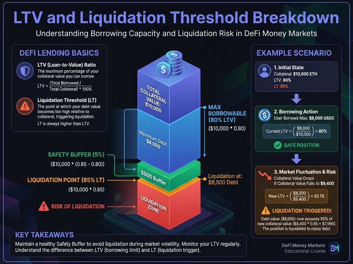
Loan-to-Value (LTV): The maximum borrowing capacity as a percentage of collateral value.
Liquidation Threshold (LT): The safety line—the collateral-to-debt ratio at which liquidation is triggered.
Understanding the Difference
This distinction is critical and often misunderstood by beginners:
LTV = Maximum Borrowing Capacity
If LTV = 80%, you can borrow up to $80 for every $100 of collateral
This is NOT the liquidation point
LT = Liquidation Trigger Point
If LT = 85%, liquidation occurs when your debt equals 85% of collateral value
This is the actual danger line
The Safety Buffer = LT - LTV
Example: ETH Collateral Position
Initial Setup:
Collateral: $10,000 worth of ETH
Maximum LTV: 80%
Liquidation Threshold: 85%
Maximum Borrowing:
Maximum borrow = $10,000 × 0.80 = $8,000
Safety Buffer:
Buffer = $10,000 × (0.85 - 0.80) = $500
This means you have a $500 cushion before liquidation
What Happens as Price Moves:
If ETH drops to $9,500: Collateral value = $9,500, debt = $8,000
Debt ratio = $8,000 ÷ $9,500 = 84.2% (still safe)
If ETH drops to $9,411: Collateral value = $9,411, debt = $8,000
Debt ratio = $8,000 ÷ $9,411 = 85% (LIQUIDATION TRIGGERED)
Why Two Different Numbers?
Protocols use two thresholds to:
Prevent over-borrowing (LTV limit)
Provide liquidation buffer (LT allows for price movement between checks)
The gap between LTV and LT gives liquidators time to act before the protocol becomes insolvent.
🔢 Health Factor: Your Safety Score
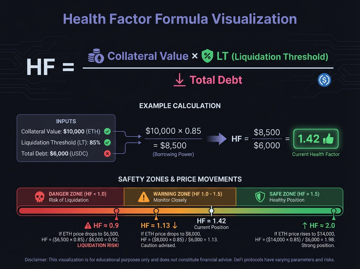
The Health Factor Formula
The Health Factor (HF) is the single most important metric when borrowing:
HealthFactor=TotalDebtCollateralValue×LiquidationThreshold
Interpreting Health Factor
HF > 1.0: Position is safe
HF = 2.0: Can withstand ~50% collateral price drop
HF = 1.5: Can withstand ~33% collateral price drop
HF = 1.1: Danger zone—any small price movement risks liquidation
HF ≤ 1.0: Position is liquidatable
HF = 1.0: Exactly at liquidation threshold
HF < 1.0: Position is underwater (should have been liquidated)
Strategic Health Factor Targets
For Beginners: HF > 2.0
Provides substantial buffer against volatility
Allows you to sleep at night
Reduces stress and monitoring frequency
For Active Traders: HF = 1.5 - 2.0
Higher capital efficiency
Requires active monitoring
Acceptable for experienced users
Danger Zone: HF < 1.3
High liquidation risk
Requires constant vigilance
Not recommended for beginners
Calculating Health Factor: Step-by-Step
Scenario: You deposit ETH and borrow USDC
Initial Position:
Collateral: 5 ETH @ $2,000/ETH = $10,000
Borrowed: $6,000 USDC
Liquidation Threshold: 85%
Health Factor Calculation: HF=$6,000$10,000×0.85=$6,000$8,500=1.42
Interpretation: HF = 1.42 means the collateral can drop ~30% before liquidation.
What Happens if ETH Drops to $1,500?
New collateral value: 5 ETH × $1,500 = $7,500
Debt remains: $6,000 (plus accrued interest)
New HF = ($7,500 × 0.85) ÷ $6,000 = $6,375 ÷ $6,000 = 1.06
Status: Still safe but approaching danger zone. You should consider adding collateral or repaying debt.
Health Factor with Multiple Collaterals
When you have multiple collateral types, the formula aggregates:
HF=TotalDebt∑(Collaterali×LTi)
Example:
Collateral 1: 3 ETH @ $2,000, LT = 85% → $5,100 effective
Collateral 2: $4,000 USDC, LT = 90% → $3,600 effective
Total Debt: $7,000 USDC
HF=$7,000$5,100+$3,600=$7,000$8,700=1.24
💧 Utilization Rate and Interest Rate Curves
What is Utilization Rate?
Utilization Rate (U) = The percentage of supplied assets currently borrowed:
U=TotalSuppliedTotalBorrowed×100%
Example:
Pool has 100 USDC supplied
60 USDC is borrowed
Utilization = 60 ÷ 100 = 60%
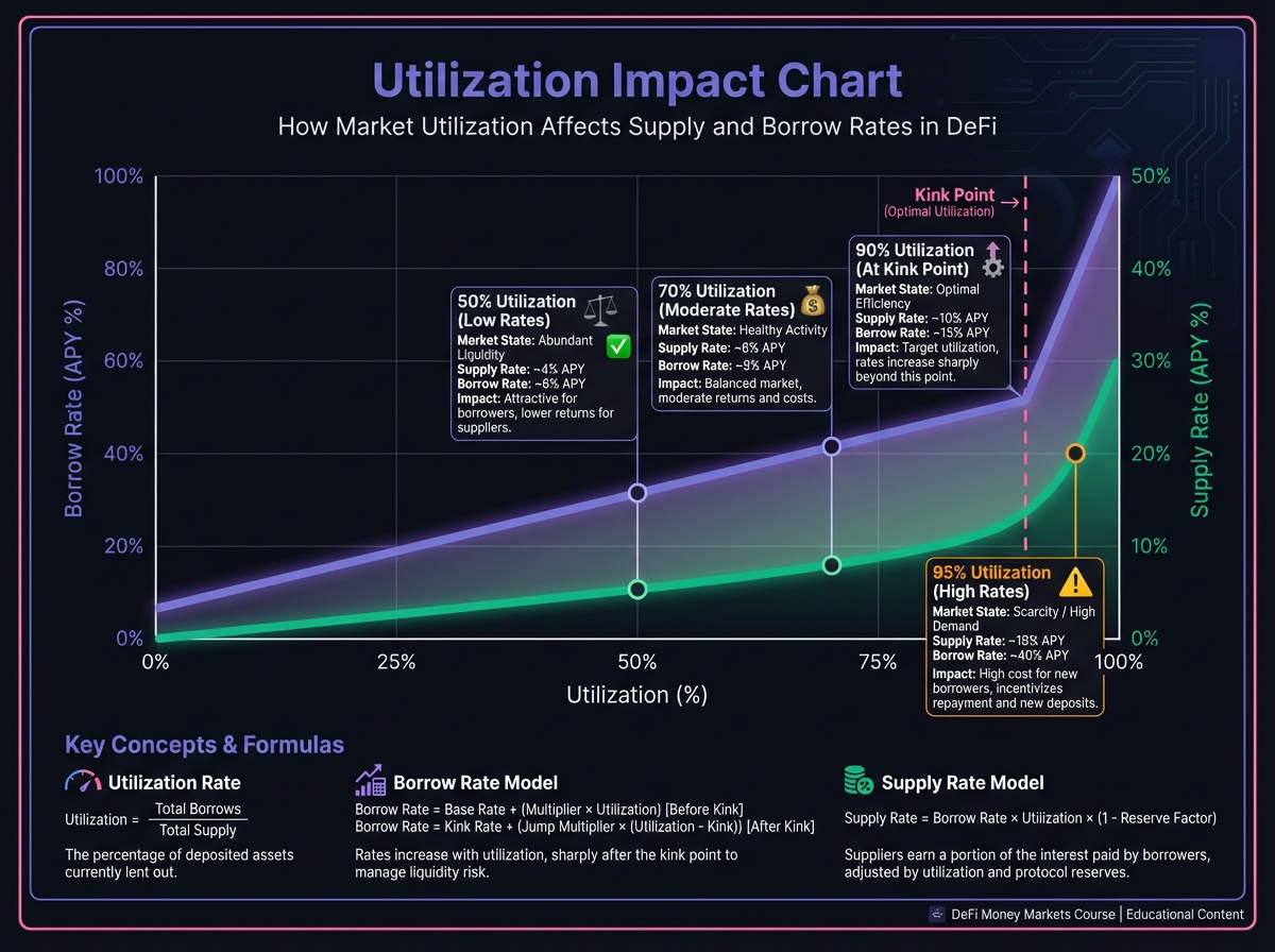
Why Utilization Matters
Utilization directly drives interest rates through the interest rate model:
Low utilization (< 50%): Lower rates (less demand, more supply)
Medium utilization (50-80%): Moderate rates (balanced)
High utilization (> 80%): Higher rates (high demand, low supply)
Very high utilization (> 90%): Extremely high rates (liquidity crisis warning)
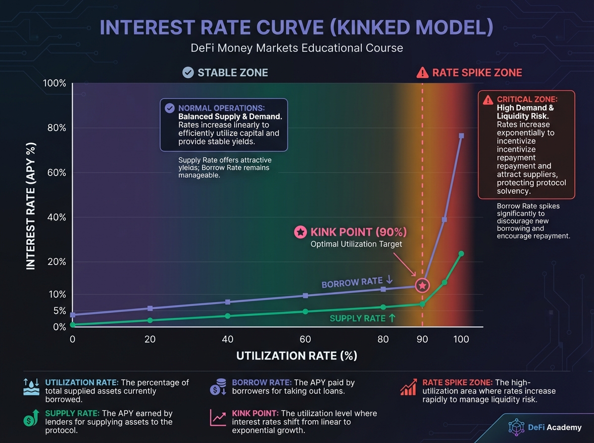
The "Kinked" Interest Rate Model
Most protocols use a kinked curve with two distinct phases:
Phase 1: Below the Kink (e.g., U < 90%)
Linear or gentle slope
Supply rate: 2-5% APY
Borrow rate: 5-8% APY
Stable and predictable
Phase 2: Above the Kink (U > 90%)
Exponential spike
Supply rate: 10-50%+ APY
Borrow rate: 50-200%+ APY
Designed to incentivize repayments
Example: Interest Rate Curve
Below Kink (U = 70%):
Supply rate: 4% APY
Borrow rate: 6% APY
Spread: 2% (to protocol reserves)
At Kink (U = 90%):
Supply rate: 5% APY
Borrow rate: 8% APY
Spread increases
Above Kink (U = 95%):
Supply rate: 15% APY
Borrow rate: 50% APY
Massive spread to attract liquidity
The Liquidity Freeze Risk
Critical Risk: If utilization reaches 100%, lenders cannot withdraw until borrowers repay.
Example Scenario:
Pool has $1M USDC supplied
$1M USDC borrowed
Utilization = 100%
You try to withdraw $10,000
Result: Transaction fails—no liquidity available
Protection Mechanisms:
Interest rate spikes incentivize repayments
High rates attract new deposits
Reserve funds (if protocol has them)
Utilization caps (max borrowing limits)
📊 Interest Rate Calculations
How Supply Rates Work
When you lend assets, you earn interest based on:
Utilization rate (how much is borrowed)
Borrow rate (what borrowers pay)
Reserve factor (protocol's cut)
Simplified Formula: SupplyRate=BorrowRate×Utilization×(1−ReserveFactor)
Example:
Borrow rate: 8% APY
Utilization: 75%
Reserve factor: 10% (protocol keeps 10%)
SupplyRate=8%×0.75×0.90=5.4%APY
How Borrow Rates Work
Borrow rates are determined by the interest rate model based on utilization:
Linear Model (simplified): BorrowRate=BaseRate+(Utilization×Slope)
Kinked Model (most common):
Below kink: Lower slope
Above kink: Steeper slope (exponential)
Accrued Interest Calculation
Interest accrues continuously, not daily or monthly.
For Lenders:
Your balance grows automatically
aToken balance increases over time
Compound effect: You earn interest on interest
For Borrowers:
Your debt increases over time
Interest compounds
Must repay principal + accrued interest
Example: Borrowing $10,000 at 6% APY:
After 1 month: Debt = $10,000 × (1 + 0.06/12) = $10,050
After 6 months: Debt = $10,000 × (1 + 0.06/2) = $10,300
After 1 year: Debt = $10,000 × 1.06 = $10,600
Key Insight: If you don't monitor your position, the debt grows even if collateral price stays the same.
🔮 The Role of Oracles
What Are Oracles?
Oracles are bridges between off-chain price data and on-chain smart contracts. They feed real-world price information (like ETH/USD) to the protocol.
Oracle Types
1. Chainlink (Push-Based)
Updates pushed to chain regularly
Industry standard for Ethereum
Highly secure and reliable
Updates every few hours or minutes
2. Pyth Network (Pull-Based)
Updates on-demand when needed
Used for high-frequency chains (Solana, Sui)
Lower latency for fast transactions
More efficient for high-throughput networks
3. Redstone (On-Demand)
Pull-based oracle
Used by some protocols for flexibility
Can provide custom data feeds
Oracle Risk
The Risk: If an oracle provides incorrect price data, the protocol makes decisions based on wrong information.
Attack Vector: Oracle manipulation via flash loans
Attacker takes large flash loan
Manipulates price on low-liquidity DEX
Oracle reads manipulated price
Protocol liquidates positions incorrectly
Attacker profits from liquidations
Protection Mechanisms:
Multiple oracle sources (e.g., Chainlink + Uniswap TWAP)
Price staleness checks (reject old prices)
Confidence intervals (require price consensus)
Circuit breakers (pause if price moves too fast)
Why Oracle Choice Matters
Different protocols use different oracles, which affects risk:
Chainlink: Most secure, but updates may lag during volatility Pyth: Fast updates, good for high-frequency chains TWAP: Smooths out manipulation but may lag behind market
For Beginners: Prefer protocols using established oracles (Chainlink) with multiple data sources.
🧮 Complete Calculation Example
Let's work through a complete example:
Initial Position Setup:
You deposit: 10 ETH @ $2,000/ETH = $20,000 collateral
Protocol parameters:
LTV: 75%
Liquidation Threshold: 80%
Interest: 5% APY borrow rate
Step 1: Calculate Maximum Borrow
Max borrow = $20,000 × 0.75 = $15,000
Step 2: Decide Borrowing Amount
You borrow: $10,000 USDC (conservative, 50% of max)
Step 3: Calculate Initial Health Factor HF=$10,000$20,000×0.80=$10,000$16,000=1.60
Step 4: After 6 Months
Scenario A: ETH Price Stable
Collateral: Still 10 ETH @ $2,000 = $20,000
Debt: $10,000 × (1 + 0.05/2) = $10,250
New HF = ($20,000 × 0.80) ÷ $10,250 = 1.56
Scenario B: ETH Rises 25%
Collateral: 10 ETH @ $2,500 = $25,000
Debt: $10,250
New HF = ($25,000 × 0.80) ÷ $10,250 = 1.95 ✅ Safer
Scenario C: ETH Drops 30%
Collateral: 10 ETH @ $1,400 = $14,000
Debt: $10,250
New HF = ($14,000 × 0.80) ÷ $10,250 = 1.09 ⚠️ Danger zone
Analysis:
Scenario A: Position safe, slight HF decline from interest
Scenario B: Position safer, can borrow more or enjoy buffer
Scenario C: Must take action—add collateral or repay debt
🎓 Beginner's Corner: Common Math Mistakes
Mistake 1: Confusing LTV with liquidation threshold
Wrong: "LTV is 80%, so I'll get liquidated at 80%"
Right: Liquidation occurs at the LT (often 85%), not LTV
Mistake 2: Ignoring accrued interest
Wrong: "My debt stays the same"
Right: Debt grows continuously. A 5% APY borrow rate means ~0.42% monthly increase
Mistake 3: Not accounting for price volatility
Wrong: "ETH won't drop 50%"
Right: Crypto is volatile. A 50% drop in a day is possible. Calculate HF at worst-case scenarios
Mistake 4: Misunderstanding utilization
Wrong: "High utilization means I earn more" (true but risky)
Right: High utilization means higher rates but also higher risk of liquidity freezes
Mistake 5: Not monitoring Health Factor
Wrong: "I'll check it monthly"
Right: Monitor daily or use alerts. Prices can move fast, and interest accrues continuously.
🔬 Advanced Deep-Dive: Dynamic Interest Rates
Adaptive Interest Rate Models
Some protocols (like Morpho) use adaptive curves that adjust automatically:
Target Utilization: The protocol targets a specific utilization (e.g., 90%)
Mechanism:
If utilization > target: Curve shifts up, rates increase
If utilization < target: Curve shifts down, rates decrease
This maintains consistent utilization levels
Formula (simplified): BorrowRate=Base+(Utilization−Target)×Sensitivity
Result: Markets maintain high utilization (efficient capital use) while keeping rates reasonable.
Compounding Frequency
Interest can compound at different frequencies:
Continuous Compounding (most DeFi):
Interest accrues every block
Formula: $A = P \times e^{rt}$
Most accurate representation
Block-by-Block:
Interest calculated per block
Updates continuously
Standard for on-chain protocols
Daily Compounding:
Interest calculated daily
Less accurate but simpler
Rare in modern DeFi
📈 Real-World Calculation: Aave USDC Market
Market State:
Total Supplied: $500,000,000 USDC
Total Borrowed: $350,000,000 USDC
Utilization: 70%
Interest Rates (at 70% utilization):
Supply APY: 4.5%
Borrow APY: 6.5%
Spread: 2% (to Aave reserves)
Your Position:
You supply: $10,000 USDC
Daily earnings: $10,000 × 0.045 ÷ 365 = $1.23/day
Monthly earnings: $1.23 × 30 = $37/month
Annual earnings: $450/year
If Utilization Spikes to 95%:
Supply APY: 12% (estimated)
Borrow APY: 45% (estimated)
Your new daily earnings: $10,000 × 0.12 ÷ 365 = $3.29/day
Trade-off: Higher yields but increased risk of liquidity freeze if utilization hits 100%.
🔧 Interactive Tools
Interactive Health Factor Calculator
Practice calculating Health Factor, LTV, and liquidation prices with this interactive tool:
Launch Lending Borrowing Calculator →
🔑 Key Takeaways
LTV vs LT: LTV is maximum borrowing; LT is liquidation trigger—they're different!
Health Factor is your safety score—keep it > 1.5 (ideally > 2.0)
Utilization drives rates: High utilization = high yields but high risk
Interest accrues continuously: Debt grows even if prices don't move
Oracles are critical: Wrong prices lead to wrong liquidations
Monitor regularly: Prices and interest change constantly
🚀 Next Steps
Now that you understand the mathematics, Lesson 3 will show you the risks in detail—liquidation mechanics, how to protect yourself, and what to avoid.
Complete Exercise 2 to practice these calculations and build your mathematical intuition.
Remember: Math protects your capital. Master these formulas, and you'll make informed decisions. Ignore them, and you'll risk liquidation or miss profitable opportunities.
← Back to Summary | Next: Exercise 2 → | Previous: Lesson 1 ←
Last updated